Using Oscilloscope Histograms to Analyze Jitter and Random Variation

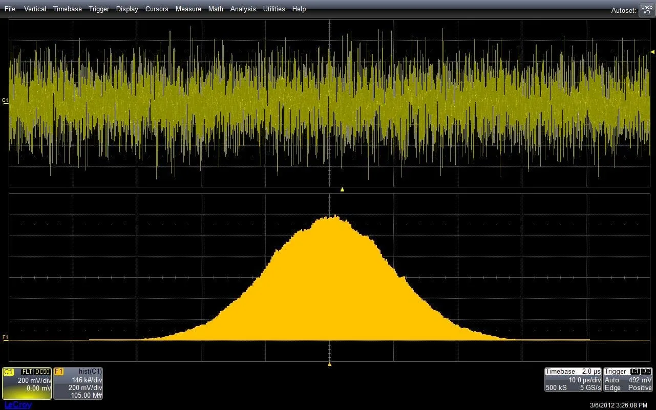
Why it matters: A single waveform capture tells you what happened once. A histogram tells you what happens statistically—across thousands or millions of acquisitions—which is exactly the view engineers need when a "random" timing or amplitude problem is actually a specific, identifiable circuit behaviour hiding in plain sight.

What a Histogram Measurement Actually Shows

Most oscilloscopes, including the Teledyne LeCroy instruments Primeasure supports across India, can take any measured parameter—period, pulse width, amplitude, rise time, or Time Interval Error (TIE)—and bin the accumulated results into a histogram. Instead of a single mean and standard deviation, you get the full shape of the distribution: where values cluster, how symmetric they are, and whether the population is unimodal or split across multiple peaks.

That shape is diagnostic. Different underlying physical processes produce recognisably different distribution shapes, so a histogram often points directly at a root cause that a track or a raw waveform would leave ambiguous.

Reading the Shape of the Distribution

• Gaussian (normal) distribution: A symmetric, bell-shaped histogram is the signature of a purely random process—thermal noise, random jitter (RJ), or other uncorrelated amplitude variation. This is the baseline shape engineers expect from a clean, well-behaved signal path.
• Rayleigh distribution: A skewed, one-sided distribution typically appears when Gaussian noise passes through a nonlinear operation, such as envelope detection or full-wave rectification. Seeing a Rayleigh shape where a Gaussian was expected is a strong clue that a nonlinear stage is reshaping the underlying noise.
• Uniform distribution: A flat-topped histogram, with roughly equal probability across a bounded range, is characteristic of timing synchronizer and arbiter circuits, where an asynchronous event is being resolved against a clock edge. The width of the flat region maps directly to the resolution window of the synchronizing circuit.
• Bimodal or multi-modal distributions: Two or more distinct peaks usually indicate two or more deterministic contributors superimposed on the same measurement—duty-cycle distortion, a crosstalk aggressor switching intermittently, or a data-dependent jitter component correlated with pattern content.

A Practical Example: Timing Synchronizer Behaviour

Consider a 400 MHz clock domain-crossing circuit where an asynchronous input is resampled by a synchronizer. Measuring the timing error between the input transition and the resolved output across a long acquisition run typically produces a uniform histogram bounded by the synchronizer's setup and hold window—not a Gaussian one. Engineers who assume every timing measurement should be Gaussian can misinterpret this as excessive jitter, when it is in fact the synchronizer behaving exactly as designed. Recognising the uniform shape for what it is avoids chasing a problem that does not exist.

Catching Rare Events That a Trace-by-Trace View Misses

The real value of histogram analysis shows up in the tails, not the peak. In serial data and clocking applications, the failures that matter—bit errors, marginal setup violations, occasional glitches—often occur at rates of one in a million or lower. No amount of scrolling through individual waveforms will reliably catch that. A histogram accumulated over a sufficiently long acquisition quantifies exactly how often a parameter exceeds a given threshold, turning "does this ever happen" into a measured percentage engineers can compare against a specification or a bit-error-rate target.

Combining histograms with infinite persistence display reinforces this: the persistence view shows where the outliers physically sit relative to the main population, while the histogram quantifies how often they occur.

Primeasure POV

• Before troubleshooting a "jitter" or "noise" problem, generate a histogram on the parameter in question—the distribution shape often tells you which category of root cause to investigate before you touch a single component.
• Don't assume Gaussian by default. Synchronizer, arbiter, and PWM-related timing measurements are frequently uniform or multi-modal by design; misreading these as random jitter wastes debug time.
• For BER-sensitive interfaces, run histograms over long acquisitions and quantify tail population directly rather than relying on a mean and standard deviation, which can understate rare-event risk.
• Teledyne LeCroy oscilloscopes pair histogram measurements directly with SDAIII jitter decomposition, letting you move from "the distribution looks unusual" to a quantified breakdown of random, deterministic, and periodic components in the same workflow.